Anatomy of the transfer matrix

The method collapses an entire layered stack into a single $4\times4$ matrix, and every reflectance and transmittance number is read straight off it. This page explains what that matrix is and what each of its elements means.

transfer returns a TransferResult of $R$/$T$ values; the matrix itself is the first item returned by the internal TransferMatrix.propagate:

M, S, Ds, Ps, γs = TransferMatrix.propagate(1.0, layers; θ=0.3)
M  # the 4×4 complex transfer matrix for the whole stack

What the matrix represents

$M$ connects the four plane-wave mode amplitudes on the two sides of the stack:

\[\psi_\text{inc} = M\,\psi_\text{sub}, \qquad \psi = \begin{pmatrix} p^{+} \\ p^{-} \\ s^{+} \\ s^{-} \end{pmatrix},\]

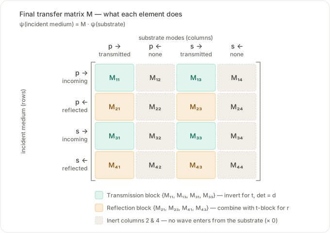
where $+$ is the forward ($+z$) mode and $-$ the backward ($-z$) mode of each polarization. Rows index modes in the incident medium; columns index modes in the substrate. On the incident side the forward modes are the incoming wave and the backward modes are the reflected wave; on the substrate side the forward modes are the transmitted wave and the backward modes are absent — nothing illuminates the stack from behind.

Which elements carry the physics

Because the backward-substrate amplitudes are zero, columns 2 and 4 multiply zero and never affect an observable — only columns 1 and 3 act. The active elements split into two blocks.

Transmission block — rows $\{1,3\}$ × columns $\{1,3\}$. Its determinant is the shared denominator, and its inverse is the transmission Jones matrix:

\[d = M_{11}M_{33} - M_{13}M_{31},\]

\[t_{pp} = \frac{M_{33}}{d}, \quad t_{ss} = \frac{M_{11}}{d}, \quad t_{ps} = -\frac{M_{31}}{d}, \quad t_{sp} = -\frac{M_{13}}{d}.\]

Reflection block — rows $\{2,4\}$ × columns $\{1,3\}$, read out against the same transmission block:

\[\begin{aligned} r_{pp} &= \frac{M_{21}M_{33} - M_{23}M_{31}}{d}, & r_{ss} &= \frac{M_{11}M_{43} - M_{41}M_{13}}{d}, \\[4pt] r_{ps} &= \frac{M_{41}M_{33} - M_{43}M_{31}}{d}, & r_{sp} &= \frac{M_{11}M_{23} - M_{21}M_{13}}{d}. \end{aligned}\]

Reflectance is then $R = |r|^2$ directly, while every transmittance $T$ — co- and cross-polarized alike — is a Poynting-vector flux ratio rather than $|t|^2$ (the transmitted wave lives in a different medium): each channel is the flux of one substrate eigenmode, evaluated with its own wavevector — see Physics Validation. The amplitude formulas above are exactly what calculate_tr evaluates.

The full $16$-element map:

Isotropic limit: Yeh's 2×2 matrices

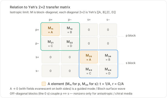
The field ordering $(p^{+}, p^{-}, s^{+}, s^{-})$ keeps the two p-modes adjacent and the two s-modes adjacent. So for isotropic (or optic-axis-aligned) media, where p and s do not mix, $M$ is block-diagonal, and each diagonal $2\times2$ block is Yeh's transfer matrix for that polarization:

\[\begin{pmatrix} A & B \\ C & D \end{pmatrix}, \qquad A = M_{11}\ (\text{p}), \quad A = M_{33}\ (\text{s}).\]

With no backward wave in the substrate, Yeh's relation gives $t = 1/A$ and $r = C/A$ — which is exactly the block formulas above specialized to $M_{13}=M_{31}=0$ (so $d = M_{11}M_{33}$, $t_{pp}=1/M_{11}$, $r_{pp}=M_{21}/M_{11}$, and likewise for s).

Bound modes and Bloch surface waves

A guided (bound) mode is a pole of $r$ and $t$ — a self-sustaining field with no incident wave — i.e. the denominator vanishes. In the decoupled case that is $A = 0$: $M_{11}=0$ for a p-polarized mode, $M_{33}=0$ for an s-polarized mode (in the full coupled problem it generalizes to $d=0$).

A Bloch surface wave (BSW) is the bound mode at the truncation of a periodic multilayer (e.g. a DBR). It lives inside a photonic band gap of the stack — so it decays into the periodic side — and below the light line of the outer cladding — so it decays into the cladding. To find one with this package:

1. Use a high-index coupling prism as the incident (first) layer so that the in-plane wavevector $\beta = k_0\,\xi$ can exceed the cladding light line.
2. Scan angle/wavelength with sweep_angle past the critical angle; the BSW appears as a sharp dip in the reflectance ($R_{pp}$ or $R_{ss}$) where $A$ passes through its zero.
3. Confirm it with efield: the field is localized and strongly enhanced at the truncation surface.

Anisotropic and chiral media

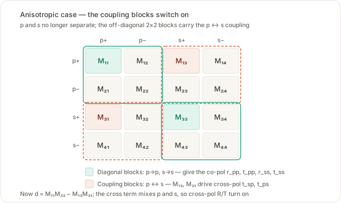
When the media are anisotropic or chiral, p and s couple and the off-diagonal blocks switch on. The elements $M_{13}$ and $M_{31}$ drive the cross-polarized transmission ($t_{sp} = -M_{13}/d$, $t_{ps} = -M_{31}/d$), and the determinant picks up the cross term:

\[d = M_{11}M_{33} - M_{13}M_{31}.\]

That cross term ties the p and s poles together, so a bound mode at $d = 0$ is generally a mixed-polarization surface mode rather than a pure p or s one. The cross-polarization observables $R_{ps}, R_{sp}, T_{ps}, T_{sp}$ — exactly zero for isotropic media — become nonzero; this same coupling is what the Circular-polarization basis output reflects.

Numerical backends: method

transfer, amplitude_coefficients, sweep_angle, and sweep_thickness accept method:

• :auto (default) uses the 2×2 :decoupled path whenever s and p cannot mix at the requested point, and :exp otherwise. You do not need to choose: results agree to ~1e-12 either way, and decoupled stacks run roughly 10× faster.
• :decoupled forces the 2×2 path and throws an ArgumentError if the stack couples s and p.
• :exp propagates each interior layer with the matrix exponential of the Berreman Δ matrix. It avoids eigenmode sorting entirely, so it is degeneracy-immune and handles near-degenerate or mixed propagating/evanescent interior layers robustly.
• :eig is the eigenmode/dynamical-matrix path, kept as an independent cross-check (transfer(λ, layers; method=:eig)).

When the 2×2 path applies

Write Berreman's field vector as $(E_x, H_y, E_y, -H_x)$. The first pair is the p wave and the second the s wave, and the off-diagonal blocks of Δ that couple them contain only $ε_{xy}, ε_{yx}, ε_{yz}, ε_{zy}$ (and the same μ elements). If those vanish in every layer, Δ is block-diagonal, so is every layer's propagator and so is their product: the whole $4\times4$ problem is two independent $2\times2$ problems, each with a closed-form propagator, and the cross-polarized coefficients are exactly zero. :decoupled requires:

• an isotropic, non-magnetic ambient and substrate;
• interior layers in which y is a principal axis of the lab-frame ε and μ;
• conductive sheets with $σ_{xy} = σ_{yx} = 0$.

The second condition covers isotropic layers and unrotated anisotropic layers, which get closed-form blocks straight from the principal values. It also covers a uniaxial optic axis tilted in the plane of incidence (Euler angles $(0, θ, 0)$ or $(π, θ, 0)$) or along y ($(π/2, π/2, 0)$), a biaxial crystal rotated about y, and μ with gyration axis y (gyrotropic_tensor(...; axis=:y), the transverse magneto-optic geometry). For these the p block gains diagonal terms ($ε_{xz}$, antisymmetric $μ_{xz}$), so the forward and backward p waves need no longer be mirror images, but each block still has a closed-form exponential. Such layers are checked numerically at every point, because a coupling that enters only through the in-plane wavevector ($ε_{yz}$, $μ_{yz}$, for example an optic axis in the yz plane) vanishes at normal incidence and nowhere else.

Everything else uses the $4\times4$ path: an optic axis with both x and y components (waveplates), μ with gyration axis z, gyration axis x away from normal incidence, and Hall-type sheets. isdecoupled(λ, layers; θ, sheets) reports which path :auto takes.

The two $4\times4$ paths agree to ~1e-12. They treat the semi-infinite ambient and substrate by eigenmodes, so the boundary limitations (anisotropic ambient, issue #71; anisotropic substrate under total internal reflection, issue #107) apply to both.

See the bibliography ("Matrix-exponential layer propagator") for references.